About me and why I created this physics website.

Rigid Body Dynamics

Two-Dimensional Rigid Body Dynamics

For two-dimensional rigid body dynamics problems, the body experiences motion in one plane, due to forces acting in that plane.

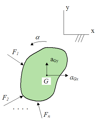
A general rigid body subjected to arbitrary forces in two dimensions is shown below.





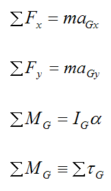
The full set of scalar equations describing the motion of the body are:




Where:

m is the mass of the body

ΣF_x is the sum of the forces in the x-direction

ΣF_y is the sum of the forces in the y-direction

a_Gx is the acceleration of the center of mass G in the x-direction, with respect to an inertial reference frame xyz, which is the ground in this case

a_Gy is the acceleration of the center of mass G in the y-direction, with respect to ground

α is the angular acceleration of the rigid body with respect to ground

ΣM_G is the sum of the moments about an axis passing through the center of mass G (in the z-direction, pointing out of the page). This is defined as the sum of the torque Στ due to the forces acting on the body (about an axis passing through the center of mass G, and pointing in the z-direction). Using ΣM_G is simply a different naming convention.

I_G is the rotational inertia of the rigid body about an axis passing through the center of mass G, and pointing in the z-direction (out of the page)


Note that, if the rigid body were rotating about a fixed point O, the final moment equation would retain the same form if we were to choose point O instead of point G. So, the equation would become:





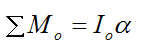
The figure below illustrates this situation.



Where the point O is a fixed point, attached to ground. A specific example of this would be a pendulum swinging about a fixed point.


Here are some examples of problems solved using two-dimensional rigid body dynamics equations:

The Physics Of A Golf Swing
Trebuchet Physics


Three-Dimensional Rigid Body Dynamics

For three-dimensional rigid body dynamics problems, the body experiences motion in all three dimensions, due to forces acting in all three dimensions. This is the most general case for a rigid body.

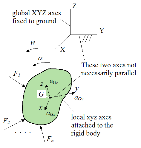
A general rigid body subjected to arbitrary forces in three dimensions is shown below.





The first three of the six scalar equations describing the motion of the body are force equations. They are:




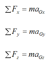
Where:

a_Gx is the acceleration of the center of mass G in the x-direction, with respect to ground (an inertial reference frame)

a_Gy is the acceleration of the center of mass G in the y-direction, with respect to ground

a_Gz is the acceleration of the center of mass G in the z-direction, with respect to ground


Note that the subscripts x,y,z indicate that the quantities are resolved along the xyz axes. For example, a force acting along the Z-axis is resolved into its components along the xyz axes in the above three equations. This can generally be done using trigonometry.

However, it is not necessary to resolve the quantities along the xyz axis. For the above three force equations, one can resolve the quantities along the XYZ axes instead.


To solve three-dimensional rigid body dynamics problems it is necessary to calculate six inertia terms for the rigid body, corresponding to the extra complexity of the three dimensional system. To do this, it is necessary to define a local xyz axes which lies within the rigid body and is attached to it (as shown in the figure above), so that it moves with the body. The six inertia terms are calculated with respect to xyz and depend on the orientation of xyz relative to the rigid body. So, a different orientation of xyz (relative to the rigid body) will result in different inertia terms. The reason that xyz is said to "move with the body" is because the inertia terms will not change with time as the body moves. So you only need to calculate the inertia terms once, at the initial position of the rigid body, and you are done. This has the advantage of keeping the mathematics as simple as possible. An added benefit of having xyz move with the rigid body is when simulating the motion of the body, over time. We can track the orientation of the body by tracking the orientation of xyz (since they move together).


For two-dimensional rigid body dynamics problems there is only one inertia term to consider, and it is I_G, as given above. For these problems I_G can be calculated with respect to any orientation of the rigid body, and it will always be the same, since the problem is planar. Therefore, we don't need to define an axes xyz that is attached to the rigid body, and has a certain orientation relative to it (like we do in three-dimensional problems). This is because, for planar problems (where motion is in one plane), I_G would be independent of the orientation of xyz (relative to the rigid body).


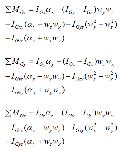
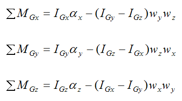
For the general case (where we have an arbitrary orientation of xyz within the rigid body), the last three equations describing the motion of the rigid body are moment (torque) equations. They are:




Where:

ΣM_Gx is the sum of the moments about the x-axis, passing through the center of mass G

ΣM_Gy is the sum of the moments about the y-axis, passing through the center of mass G

ΣM_Gz is the sum of the moments about the z-axis, passing through the center of mass G

w_x, w_y, w_z are the components of the angular velocity of the rigid body with respect to ground, and resolved along the local xyz axes. To calculate these components, one must first determine the angular velocity vector of the rigid body with respect to the global XYZ axes, and then resolve this vector along the x, y, z directions to find the components w_x, w_y, w_z. This is often done using trigonometry.

α_x, α_y, α_z are the components of the angular acceleration of the rigid body with respect to ground, and resolved along the local xyz axes. To calculate these components, one must first determine the angular acceleration vector of the rigid body with respect to the global XYZ axes, and then resolve this vector along the x, y, z directions to find the components α_x, α_y, α_z. This is often done using trigonometry.

I_Gx is the rotational inertia of the rigid body about the x-axis, passing through the center of mass G

I_Gy is the rotational inertia of the rigid body about the y-axis, passing through the center of mass G

I_Gz is the rotational inertia of the rigid body about the z-axis, passing through the center of mass G

I_Gxy is the product of inertia (xy) of the rigid body, relative to xyz

I_Gyz is the product of inertia (yz) of the rigid body, relative to xyz

I_Gzx is the product of inertia (zx) of the rigid body, relative to xyz


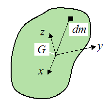
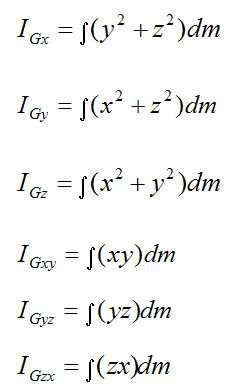
The six inertia terms are evaluated as follows, using integration:







The orientation of xyz relative to the rigid body can be chosen such that





This orientation is defined as the principal direction of xyz.

With this simplification, the moment equations become:




These are known as the Euler equations of motion. Clearly, it is a good idea to choose the orientation of xyz so that it lies in the principal direction. For every rigid body a principal direction exists. If a body has two or three planes of symmetry, the principal directions will be aligned with these planes. For the case where there are no symmetry planes in the body, the principal direction can still be found, but it involves solving a rather complicated cubic equation.

Note that, for the three moment equations and six inertia terms, their quantities must be with respect to the xyz axes (this is unlike the first three force equations, where this is optional). For the inertia terms, the reason for this is obvious since this is how they are defined. But for the moment equations, the reason is rather complicated, but basically it comes down to how they are derived, which is discussed here.

For example, a moment acting about the Y-axis must be resolved into its components along the xyz axes in order to use the above moment equations. This can generally be done using trigonometry.


Note that, if the rigid body were rotating about a fixed point O, the above moment equations and six inertia terms would retain the same form if we were to choose point O instead of point G. You just replace the subscript G with the subscript O, and everything else stays the same. Note that the xyz axes would have origin at point O instead of point G.

The figure below illustrates this situation.




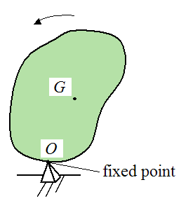
Where the point O is a fixed point, attached to ground. A specific example of this would be a spinning top precessing around a fixed point.


For two-dimensional rigid body dynamics problems the angular acceleration vector is always pointing in the same direction as the angular velocity vector. However, for three-dimensional rigid body dynamics problems these vectors might be pointing in different directions, as shown below.




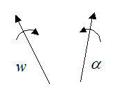
These vectors can be expressed as:



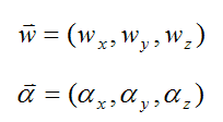
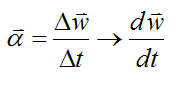
In two-dimensions, to find the angular acceleration you simply differentiate the magnitude of the angular velocity, with respect to time. In three-dimensions you have to account for the change in magnitude and direction of the angular velocity vector (since both might change with time), so this does complicate matters a bit. This is done by calculating the difference in the angular velocity vector over a very small time step Δt, where Δt→0. To illustrate, see the figure below.




Using calculus, the angular acceleration is calculated as follows (taking the limit as Δt→0):





The three force equations, and three moment equations shown here for three-dimensional rigid body dynamics problems "fully describe" all possible rigid body motion. They comprise the full set of equations you need to solve the most general rigid body dynamics problems. All simplifications can be made from these six equations. For example, if one assumes planar motion, the six equations reduce to the two-dimensional dynamics equations given above.


Note that the positive directions of the individual X, Y, Z axes are in the directions shown in the first figure. Similarly, the positive directions of the individual x, y, z axes are also in the directions shown in the first figure. This choice of sign convention is important when using the rigid body dynamics equations given here (especially the moment equations). This is explained on the equations of motion page.


For additional background information see:

Parallel Axis And Parallel Plane Theorem
A Closer Look At Velocity And Acceleration


Here are some examples of problems solved using three-dimensional rigid body dynamics equations:

The Physics Of Bowling
Euler's Disk Physics
Gyroscope Physics

To gain more insight into rigid body dynamics see Mechanical Waves.



Return to Useful Physics Formulas page


Return to Real World Physics Problems home page