Heat Exchanger
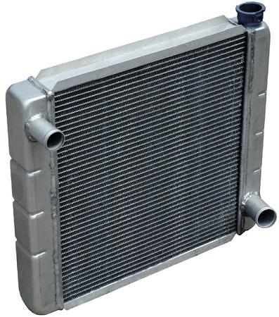
Automobile Radiator. Source: http://en.wikipedia.org/wiki/Radiator. Author: http://en.wikipedia.org/wiki/User:Bill_Wrigley
The heat exchanger is a very important device used in many real world applications in which heat must be transferred from one medium to another. In many cases, the two mediums are separated by a solid wall, although in some cases the two mediums are in direct contact with each other, so that mixing occurs. For example, in some applications steam is injected into water in order to heat it up.
Some common applications where a heat exchanger is used are: refrigeration, air conditioning, space heating, and power plants, to name a few. There are of course many more.
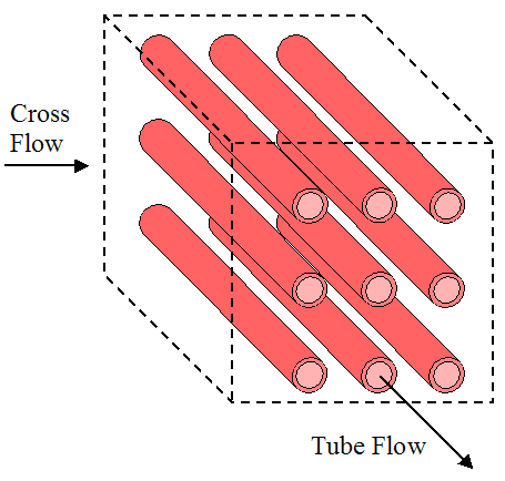
There is a large variety of heat exchanger configurations, but most can be categorized into one of three types. The three types are: Parallel-flow or counterflow configuration, cross-flow configuration, and shell-and-tube configuration.
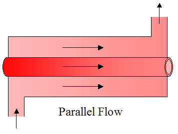
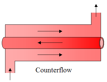
Parallel flow and counterflow configurations are shown in the two figures below. Both figures show a simple concentric tube arrangement in which one of the fluids flows on the inner tube and the other fluid flows in the annular gap (between the tubes). The figures show the hot fluid as being inside the inner tube, and the cold fluid as being inside the annular gap. In the parallel flow configuration both the hot and cold fluids flow in the same direction. In the counterflow configuration the fluids flow in opposite directions. These will be discussed in more detail later.
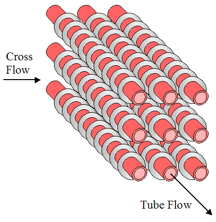
Heat transfer is usually better when a flow moves across tubes than along their length. Hence, cross-flow is often the preferred flow direction, and tends to be better than parallel flow or counterflow configurations. Cross flow configurations are shown in the three figures below. The first figure shows cross flow over an unfinned array of tubes. The second and third figures show cross flow over a finned array of tubes, with square fins and circular fins (as shown). The purpose of fins is to increase heat transfer between the hot and cold mediums. This will be discussed in more detail later.
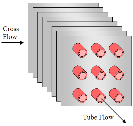
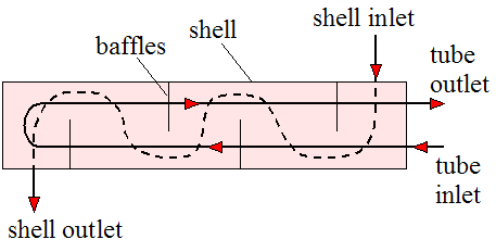
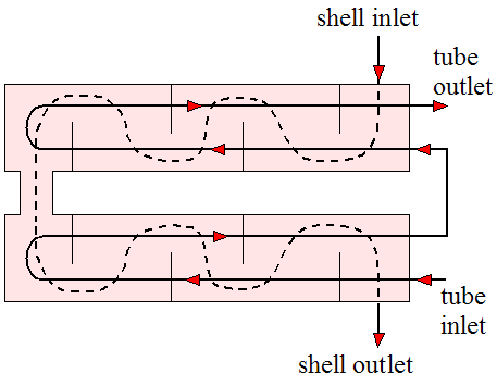
Shell-and-tube configurations are shown in the three figures below. One of the fluids flows through the inside of the shell and the other fluid flows through tubes passing through the inside of the shell, thereby enabling heat transfer between the two fluids. Baffles are added to enhance the convection coefficient, which increases heat transfer between the two fluids. The baffles serve to induce turbulent mixing and a cross-flow component, both of which increase the convection coefficient. The first figure shows one shell pass and two tube passes. The second figure shows two shell passes and four tube passes. The third figure shows a more detailed drawing of a shell-and-tube heat exchanger with one shell pass and one tube pass.
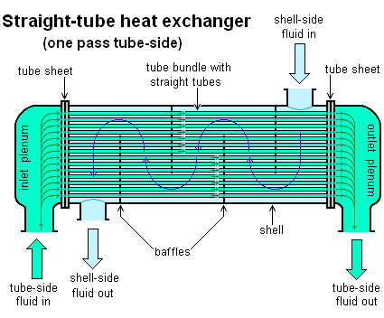
Source: http://en.wikipedia.org/wiki/Heat_exchanger. Author: http://commons.wikimedia.org/wiki/User:H_Padleckas
In the next section we will explain how fins are used to increase the heat transfer in a heat exchanger, thus boosting its effectiveness.
Increasing Heat Transfer In Heat Exchangers Using Fins
A fin can be thought of as an extension of a surface. It adds additional surface area, which enables additional heat flow to or from the medium the fin is in contact with, by way of convection. To illustrate in quantitative terms the usefulness of a fin consider the following schematic showing a pin fin protruding out of a base surface at surface temperature Tb. A differential element of width dx is shown in orange. It will be necessary to consider this element for the analysis that follows, which uses calculus.
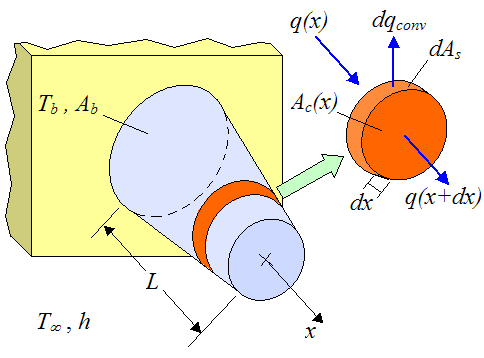
Where:
Ab is the area of the pin fin at its base
L is the length of the fin (in the x-direction)
T∞ is the temperature of the ambient environment (assumed constant everywhere)
h is the convection coefficient between the fin and the ambient environment (assumed constant)
Ac(x) is the cross-sectional area of the fin at position x
dAs is the surface area around the perimeter of the differential element, at position x
dqconv is the heat flow rate from the surface area around the perimeter of the differential element, by convection, at position x
q(x) is the heat flow rate into the element at position x, by conduction
q(x+dx) is the heat flow rate out of the element at position x+dx, by conduction
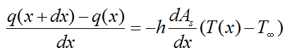
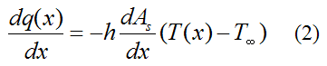
Assume steady state heat flow where the energy that enters the differential element equals the energy that exits the differential element. This is a valid assumption for steady state operating conditions.
We can write the energy balance as
The left side of the above equation is the heat energy entering the differential element. The right side of the above equation is the heat energy exiting the differential element.
By Newton’s law of cooling,
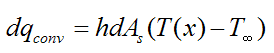
where T(x) is the fin temperature at position x.
Substitute the above equation into equation (1). We get
Rearrange the above equation to give
Divide both sides of the above equation by dx. We get
For dx→0 this becomes
From Fourier’s law,
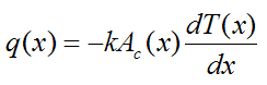
where k is the thermal conductivity of the fin material (assumed constant throughout the material).
Substitute the above equation into equation (2), and simplify. This gives us the final general differential equation for one-dimensional steady state heat transfer from an extended surface (given below). Using this equation we can solve for the temperature distribution T(x) given some set of boundary conditions.
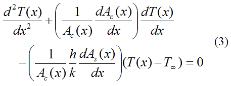
Note that although h and k are treated here as constant, this is not necessarily the case. But it is a reasonable simplification.
To get an idea of the degree to which a fin can increase heat transfer let's assume the pin fin discussed here is of constant cross-sectional area, where Ac(x) = Ac. Then, dAc(x)/dx = 0 in the above equation, and dAs(x)/dx = P, where P is the perimeter (with As(x) = Px). The above equation then becomes
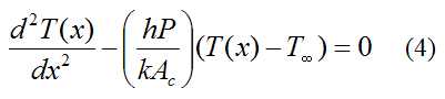
Since the above is a second order differential equation, we need two boundary conditions in terms of x to solve it. We can set the first boundary condition as T(0) = Tb. For the second boundary condition we can assume negligible heat transfer at the tip, at x = L, so that q(L) = 0. This is a good assumption for a long fin, relative to its width, since the longer the fin is, the closer its tip temperature is to the ambient temperature T∞, which means that the temperature gradient T(x) at the tip approaches zero. By Fourier's law this means that the heat flow out of the tip approaches zero.
Thus, Fourier’s law at x = L gives
so that
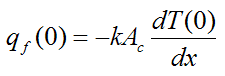
We can now solve equation (4) for the temperature distribution T(x). With this temperature distribution known we can solve for the heat transfer rate qf at the base of the fin (at x = 0).
By Fourier’s law,
Hence, solving for T(x) and substituting into the above equation we get
where
and

Note that equation (5) represents the heat transfer from the base of the surface (with area Ab = Ac) to which the fin is attached (at x = 0). In the absence of the fin the heat transfer rate from the base is simply qb where
To see how much the fin increases heat transfer calculate the following ratio:
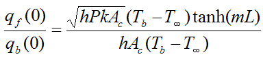
which becomes
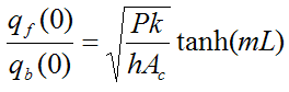
To illustrate by example, assume the pin fin is circular so that P = πd, where d is the pin fin diameter. Set d = 0.01 m, k = 180 W/m·K, h = 50 W/m2K, and L = 0.1 m.
We get
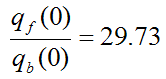
Given this high ratio, it's clearly very useful to add fins to increase heat transfer from a surface. The alternative way to increase heat transfer is by increasing h and/or decreasing T∞ which is not always practical. Hence, adding fins makes more sense. For example, radiators (as shown in the first picture on this page) have many fins since it is the only way to enable the high rate of thermal energy exchange with the air. Note that despite the name, radiators generally transfer the bulk of their heat (with some medium, such as air) via convection, not by thermal radiation, so a more accurate name for them would be "convectors". In fact, heat exchangers in general transfer the bulk of their heat via convection, and radiation heat transfer is usually negligible in comparison.
Note that the heat transfer rate qf increases for increasing k. This physically means that the temperature of the fin is closer to the base temperature Tb, along its length. In practical terms this means we want k as high as possible. Also, note that beyond a certain point, increases in L do not significantly increase the rate of heat transfer qf. This is because the farther you are along the fin, the closer the fin temperature T(x) is to T∞, which of course means a lower convective heat transfer rate from the fin to the environment (by Newton's law of cooling).
Fins are especially important for situations where the convecting medium is air or some gas (with lower h) and the surface area of the object that needs to lose (or gain) heat is (relatively) small. In this case fins will greatly aid in the transfer of heat to or from the object. If the convecting medium is a fluid, such as water, then h will generally be much higher and fins may not be necessary.
Also note that Tb can be either greater than or less than T∞. The mathematics of the solution does not change for either case. It just means that heat flows out of, or into the fin (respectively).
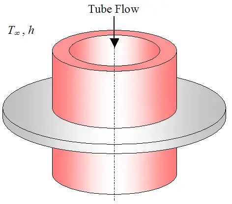
Fins can have a variety of shapes. For example, they can be pin fins protruding from a surface (as just described), or annular fins around a tube used to enhance heat flow into or out of the fluid flowing through the tube. The figure below illustrates such a fin.
If fins are attached to a wall with a metallurgical or adhesive joint, a significant thermal contact resistance may exist at the interface. This can be accounted for by a fin correction factor, discussed in a later section on the overall heat transfer coefficient.
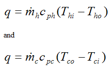
Next, we will analyze the parallel flow heat exchanger for steady state flow. Steady state flow is a valid assumption for steady operating conditions and temperatures.
Parallel Flow Heat Exchanger
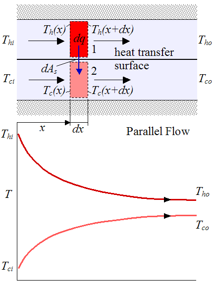
The figure below shows a schematic of a parallel-flow heat exchanger along with temperature distribution for the hot and cold fluids. We treat the heat exchanger as insulated around the outside so that the only heat transfer is between the two fluids.
As one would expect, the cold fluid (bottom curve) heats up and the hot fluid (top curve) cools down.
Where:
Thi is the temperature of the hot fluid at the inlet
Tci is the temperature of the cold fluid at the inlet
Tho is the temperature of the hot fluid at the outlet
Tco is the temperature of the cold fluid at the outlet
Th(x) is the temperature of the hot fluid at position x (left side of differential element 1. This differential element, of length dx and enclosed by dashed lines, is a control volume that is fixed in space)
Th(x+dx) is the temperature of the hot fluid at position x+dx (right side of differential element 1)
Tc(x) is the temperature of the cold fluid at position x (left side of differential element 2)
Tc(x+dx) is the temperature of the cold fluid at position x+dx (right side of differential element 2)
dAs is the differential area between differential elements 1 and 2. This differential area is located on the heat transfer surface (a wall) separating the hot and cold fluid streams.
dq is the heat flow rate between differential fluid elements 1 and 2
Assume steady state heat flow where the energy that enters the top differential element equals the energy that exits this element. We can write the energy balance as
The left side of the above equation is the energy entering the differential element. The right side of the above equation is the energy exiting the differential element.
Rewrite the above equation so that it becomes
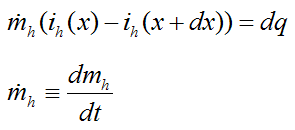
By the First law of thermodynamics the left side of the above equation can be expressed as
Where:
dmh/dt is the mass flow rate of the top (hot) fluid
ih(x) is the fluid enthalpy entering the left side of the differential element, and ih(x+dx) is the fluid enthalpy leaving the right side of the differential element. In the above equation thermal conduction along the axial (x) direction can be assumed negligible, and potential and kinetic energy changes are also assumed negligible.
If we assume constant specific heat cph for the fluid in the top differential element, and express the change in enthalpy (ih(x)−ih(x+dx)) as cph multiplied by the temperature difference across the differential element (Th(x)−Th(x+dx)), the above expression then becomes
Note that we are treating cph as constant, although it can vary as a result of temperature variations in the fluid. In this case it is reasonable to use an average value based on the average temperature of the hot fluid between the inlet and outlet.
Also note that Th(x) is the mean (average) temperature across the cross-section of the channel (at position x), for the top fluid. It is necessary to make this distinction because in real flows the temperature can vary across the cross-section.
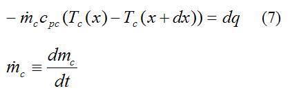
Similarly, we can also apply an energy balance to the bottom differential element. Following the same procedure as before, we get
Where:
dmc/dt is the mass flow rate of the bottom (cold) fluid
cpc is the specific heat of the fluid in the bottom differential element. We treat it as constant, although it can vary as a result of temperature variations in the fluid. In this case it is reasonable to use an average value based on the average temperature of the cold fluid between the inlet and outlet.
From Newton’s law of cooling
where U is the overall heat transfer coefficient between the top and bottom fluid. Due to variations in fluid properties and flow conditions, U may vary over the flow length. However, in many applications such variations are not significant and one can reasonably assume a constant, and average value of U.
Combining equations (6)-(8) and using calculus to solve for q we get
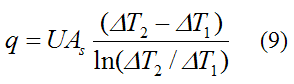
Where:
ΔT1 = Thi−Tci
ΔT2 = Tho−Tco
As is the total area of the heat transfer surface. For example, if the length of the heat transfer surface is L (in the horizontal x direction) and its depth into the page is b then As = L×b.
By direct observation, the above equation tells us that q is directly proportional to U and As. This makes sense since increasing U decreases the resistance to heat transfer thereby enabling a higher q. And increasing As increases the heat transfer surface area which also allows for a higher q.
It is worth noting that the total heat transfer rate q out of the top (hot) fluid must also equal the total heat transfer rate into the bottom (cold) fluid. Hence,
The two equations above can be used in addition to equation (9) to solve a problem involving parallel flow heat exchangers. The above two equations also apply for a counterflow heat exchanger. Note that numerical iteration may be necessary in equation (9) for cases where unknown inlet and/or outlet temperature(s) need to be solved for. However, with computers this is easy to do.
By direct observation, the above two equations tell us that q is directly proportional to dm/dt and cp. This makes sense since increasing dm/dt increases the rate of transport of energy thereby enabling a higher q. And a greater cp means that the medium can "hold" more energy per unit mass and per unit of temperature, which also allows for a higher q.
It follows that, for a given q, a higher product (dm/dt)cp for the (hot or cold) fluid means a lower temperature difference between inlet and outlet for that fluid. And a lower product (dm/dt)cp for the (hot or cold) fluid means a higher temperature difference between inlet and outlet for that fluid.
Counterflow Heat Exchanger
The figure below shows a schematic of a counterflow heat exchanger along with temperature distribution for the hot and cold fluids. Once again, we treat the heat exchanger as insulated around the outside so that the only heat transfer is between the two fluids.
As one would expect, the cold fluid (bottom curve) heats up and the hot fluid (top curve) cools down.
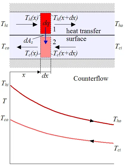
The same steps are followed to derive q for a counterflow heat exchanger as for a parallel flow heat exchanger. The only difference is that equation (7) does not have a negative sign. Equation (9) is the same as before, but with the following variables now defined differently, as follows:
ΔT1 = Thi−Tco
ΔT2 = Tho−Tci
Note that a counterflow heat exchanger is more efficient than a parallel flow heat exchanger. It takes a smaller heat transfer surface area As to achieve the same heat transfer rate q as a parallel flow heat exchanger, with all else being equal. But despite this there may be advantages to using a parallel flow heat exchanger instead of a counterflow exchanger, such as when we wish to limit the amount of heat transfer between two fluid streams.
Also note that in a counterflow heat exchanger Tco can be greater than Tho, but not for a parallel flow heat exchanger.
In principle, the maximum possible heat exchange would be achieved with a counterflow heat exhanger of infinite length. In such a heat exchanger the maximum possible temperature difference achieved (by one of the fluids) would be equal to Thi−Tci. For example, the cold fluid would be heated to the inlet temperature of the hot fluid, or the hot fluid would be cooled to the inlet temperature of the cold fluid. The maximum possible temperature difference will occur for the (hot or cold) fluid with the lowest product (dm/dt)cp. It will be this fluid which experiences the greatest temperature change between inlet and outlet. Therefore, with known inlet temperatures for both fluids, the maximum possible heat transfer rate for a counterflow heat exchanger is given by qmax = Cmin(Thi−Tci), where Cmin is the minimum of the product (dm/dt)cp for either the hot or cold fluid. By conservation of energy, the fluid with the greater product (dm/dt)cp will also experience the same rate of heat transfer qmax, but it will have a lower temperature difference between inlet and outlet since the product (dm/dt)cp is larger. Thus, it is easiest to calculate the maximum rate of heat transfer (qmax) for the (hot or cold) fluid which experiences the greatest possible temperature difference between inlet and outlet (Thi−Tci), which in turn must correspond to the fluid with the smallest product (dm/dt)cp.
Knowing qmax can be useful in making design decisions since it tells you how close your heat exchanger design is to delivering its theoretical maximum rate of heat transfer, and this in turn tells you how much improvement is possible. Keep in mind that the maximum rate of heat transfer (qmax, as given above) applies to any heat exchanger (not just a counterflow heat exchanger).
For a parallel flow or counterflow heat exchanger, if one of the (hot or cold) fluid streams is condensing or evaporating, its temperature will remain approximately constant between inlet and outlet. This constant temperature can then be applied to the equations as Tci = Tco (for the cold fluid) or Thi = Tho (for the hot fluid). These temperatures (along with other known variables) can then be substituted into equation (9) and one of the two equations shown below (which were given previously). The equation to use is the equation associated with the fluid that is not condensing or evaporating. Equation (9) and this one other equation can then be used to solve the problem. (Note that the convection coefficient for the condensing or evaporating fluid will need to be determined given its (known) condensation or evaporation temperature, and this convection coefficient will be one of the variables used to calculate the overall heat transfer coefficient, which is discussed next).
The Overall Heat Transfer Coefficient
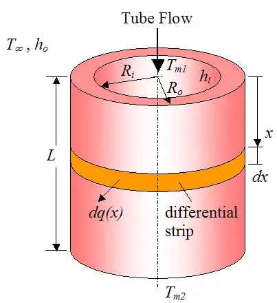
The overall heat transfer coefficient U is straightforward to calculate for steady state flow. To illustrate, consider the figure below which shows a fluid flowing through an (unfinned) tube.

Where:
hi is the internal convection coefficient
ho is the external convection coefficient
Tm1 is the mean temperature of the fluid flowing inside the tube, at the entrance. Note that this mean temperature is the average temperature of the fluid over the cross-sectional area
Tm2 is the mean temperature of the fluid flowing inside the tube, at the exit
T∞ is the ambient temperature outside the tube (assumed constant everywhere)
Ri is the inside radius of the tube
Ro is the outside radius of the tube
L is the tube length
The U value for the tube heat transfer can be calculated from the following equation:
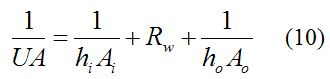
where A can either be equal to Ai or Ao, where Ai = 2πRiL and Ao = 2πRoL. The value of A can be chosen arbitrarily since the product UA will not change as a result.
Also,
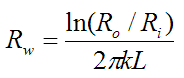
where k is the thermal conductivity of the tube (a cylinder).
Equation (10) comes from the fact that energy flow is constant (steady state) through the different mediums located between the tube fluid and the ambient. To show this, consider the schematic shown below. For visualization purposes let's imagine we have an imaginary differential strip (of thickness dx, in the x-direction) wrapping around the tube at some position x along the tube length. At this position x, heat flows outward in the radial direction through the strip at a rate dq(x). (Note that axial heat conduction (in the x direction) is assumed negligible).
We can write the following heat rate equations:
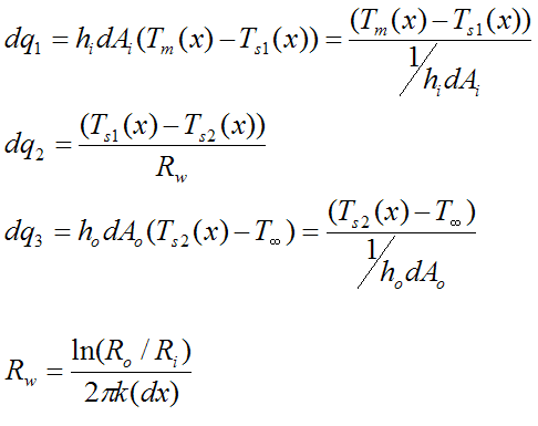
Where:
Tm(x) is the mean fluid temperature at position x
Ts1(x) is the inner wall temperature at position x
Ts2(x) is the outer wall temperature at position x
dAi is the area on the inside tube wall, at the location of the differential strip, where dAi = 2πRidx
dAo is the area on the outside tube wall, at the location of the differential strip, where dAo = 2πRodx
dq1 is the heat flow (through the differential strip) between the fluid (at mean temperature Tm(x)) and the inner tube wall (at temperature Ts1(x))
dq2 is the heat flow through the tube wall (through the differential strip), with inner wall temperature Ts1(x) and outer tube wall temperature Ts2(x)
dq3 is the heat flow (through the differential strip) between the outer tube wall (at temperature Ts2(x)) and the ambient (at temperature T∞)
For steady state heat flow,
where dq(x) is the heat flow through the differential strip at position x. Thus we can write
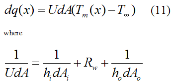
and U is defined as the overall heat transfer coefficient, which allows the heat flow rate to be expressed in a convenient and compact way, as given by equation (11).
Note that dA is chosen arbitrarily as either dAi or dAo. The above equation is a mathematical result of dq1 = dq2 = dq3.
U is a constant, independent of position x, in the above equation. To see this rewrite the above equation as
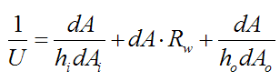
Since hi, ho, dA/dAi, dARw, and dA/dAo are all constants then U is a constant. As a result, the calculation of U from the above equation gives the same result as calculating U from Equation (10), so it’s consistent.
Note that equation (11) has the same form as equation (8) (with q = q(x)). Also, the energy balance for the fluid flow remains the same here as in equations (6) or (7). And since the ambient temperature is treated as constant here we can use equation (9) for the overall heat transfer q provided that we treat one of the fluid streams as having constant temperature throughout. Therefore, we can set Thi = Tho = T∞. Thus,
Where:
ΔT1 = T∞−Tci
ΔT2 = T∞−Tco
A positive value of q means that heat is flowing into the tube, and a negative value of q means that heat is flowing out of the tube.
For the case of a tube with fins on the inside and/or outside we can still use equation (10) but with a correction factor η now included which corrects for the presence of the fins (and any contact resistance, as mentioned earlier). Thus,
Where:
ηi is the correction factor for the inside surface of the tube, and ηo is the correction factor for the outside surface of the tube. This correction factor is between 0 and 1. For an unfinned surface η = 1.
The area on the inside of the tube (fin area plus exposed base) is equal to Ai. The area on the outside of the tube (fin area plus exposed base) is equal to Ao.
Once again, A can be chosen to be either the total surface area on the inside surface (Ai) or on the outside surface (Ao). The choice does not matter since the product UA is constant. Note that if we choose A on a side on which fins are present, then A is the total surface area comprised of the surface area all around the fins plus the surface area of the exposed base (between the fins).
The correction factors η can be found for a variety of finned surfaces (based on their shape, size, spacing, thickness, etc.) and is given in analysis books on heat exchangers, such as Compact Heat Exchangers, by Kays and London. This book is a good reference for those wanting to design or analyze finned heat exchangers.
Finally, we can add fouling factors to the above equation which accounts for deposits accumulating on the inner and outer surfaces, over time. These deposits can be a result of fluid impurities, rust, or chemical reactions between the fluid and wall material. The modified equation accounting for fouling factors then becomes
where Rfi'' is the fouling factor on the inside tube surface and Rfo'' is the fouling factor on the outside tube surface. Typical fouling factor values are given in the section on Fouling Resistance in a heat transfer textbook that I got for free online, written by John H. Lienhard (IV and V), from the Department of Mechanical Engineering, University of Houston, and Massachusetts Institute of Technology (respectively). This is also a good reference for heat exchangers and heat transfer theory. I used this book as a reference when creating this page (http://web.mit.edu/lienhard/www/ahtt.html).
Since the heat transfer q is directly proportional to the product UA (from equation 12) one would wish to maximize UA in order to maximize the rate of heat transfer.
Looking at the above equation you can only maximize UA by minimizing the above equation (1/UA). This can be done by making all the terms on the right side as small as possible (while still meeting heat exchanger design requirements). The magnitude of the above equation is limited by the largest term on the right side of the equation, whatever it works out to be (based on the parameters of the problem). So it makes sense to keep all terms as small as possible, which means keeping the fouling factors and Rw as small as possible, and using fins on the inside of the tube, if practical (such as aligned with the flow direction) and the outside of the tube, in order to increase the products ηihiAi and ηohoAo, which results in increased product UA.
For example, lets say the fouling factors and Rw are small enough to be neglected, and let’s say ηihiAi = X and ηohoAo = 5X, in which the outside tube surface is finned and the inside tube surface is unfinned (which is why ηohoAo is larger).
Now, substitute ηihiAi = X and ηohoAo = 5X into the above equation and we get UA1 ≅ (5/6)X
Now let’s say that we add fins to the inside tube surface as well so that ηihiAi and ηohoAo are comparable in magnitude so that ηihiAi ≅ ηohoAo ≅ 5X
Now, substitute ηihiAi = ηohoAo = 5X into the above equation and we get UA2 ≅ (5/2)X
UA2/UA1 = 3, which is clearly a large improvement in heat transfer by making both surfaces finned.
Estimating The Convection Coefficient h
Estimating the convection coefficient for a variety of geometries, fluid types, and flow conditions, is a difficult problem, and is by no means simple to explain in brief terms. For this reason it is best to refer to dedicated sections in books that explain in detail how to estimate convection coefficients for different configurations, along with associated pressure drop for the fluid streams. For standard finned surfaces one may refer to the book Compact Heat Exchangers listed above, to find the convection coefficients. For unfinned surfaces one may refer to the sections on convective heat transfer, as explained in the heat transfer textbook I got for free online (as mentioned above). Alternatively, you may prefer to reference a heat transfer book directly which also gives convection coefficient estimates for unfinned surfaces. A good book for this is Fundamentals of Heat and Mass Transfer, 5th Edition, by Incropera and Dewitt. The relevant sections in this book are on internal and external flow, and boiling and condensation. The fourth edition of this book was a very useful reference that I used when creating this page.
Some typical values of the convection coefficient h are:
• Free convection for gases: 2-25 W/m2K
• Free convection for liquids: 50-1000 W/m2K
• Forced convection for gases: 25-250 W/m2K
• Forced convection for liquids: 50-20,000 W/m2K
• Convection with phase change (boiling or condensation): 2500-100,000 W/m2K
The reference for the above values is from: Fundamentals of Heat and Mass Transfer, Fourth Edition, page 8, by Incropera and Dewitt, 1996.
Example Problem For Counterflow Heat Exchanger
We are given a counterflow heat exchanger with the following known values:
cpc = 4200 J/kg·K
cph = 1000 J/kg·K
dmc/dt = 1 kg/s
dmh/dt = 1.7 kg/s
Tci = 40 degrees Celsius
Thi = 280 degrees Celsius
As = 0.7 m2 (heat transfer surface area)
Rw = 4.0 × 10⁻⁵ K/W (wall thermal resistance)
hc = 1000 W/m2K (convection coefficient for cold fluid)
hh = 250 W/m2K (convection coefficient for hot fluid)
Assume that the heat transfer surface area on the cold and hot side are approximately equal.
Find the outlet temperature of the hot and cold fluid and the rate of heat transfer (q) between them.
Solution
There are three unknowns to solve for. They are Tco, Tho, and q. We need three equations to solve for these three unknowns.
The first equation to use represents the heat transfer rate (q) into the cold fluid: q = (dmc/dt)cpc(Tco−Tci)
The second equation to use represents the heat transfer rate (q) out of the hot fluid. This is equal to the heat transfer rate into the cold fluid. The equation is: q = (dmh/dt)cph(Thi−Tho)
The third equation to use is given by equation (9), with the following variables defined as follows for a counterflow heat exchanger:
ΔT1 = Thi−Tco
ΔT2 = Tho−Tci
To calculate U we can use equation (10). With hi ≡ hc and ho ≡ hh this gives a value of U = 198.89 W/m2K.
Solving numerically, we get Tco = 47.5 degrees C, Tho = 261.4 degrees C, and q = 31590 W.
Heat Exchanger Design
To choose a suitable heat exchanger for a certain application requires a level of knowledge and experience. The information presented here along with the books referenced here is certainly a good start. When designing or choosing a heat exchanger there is no single "correct" solution. Different types of heat exchangers can work equally well.
There are different ways to optimize heat exchanger design. Part of the optimization usually requires that the tube wall thickness be as small as possible (while still being strong enough), and the thermal conductivity of the tube material be as high as possible. This ensures that the thermal resistance of the tube wall is as low as possible which aids in heat transfer. Also, we wish to keep the pressure drop of the hot and cold fluid streams between inlet and outlet as small as possible. However, to increase the rate of heat exchange between the two streams we must increase the convection coefficient (h), by either adding fins, increasing surface roughness, increasing tube length and/or decreasing tube diameter. But this unavoidably increases the pressure drop and consequently increases the pump power requirements to overcome the flow resistance associated with this pressure drop. Hence, good heat exchanger design must be a tradeoff between pressure drop and good heat exchange. In some cases, such as for shell-and-tube heat exchangers, it may be possible to minimize pressure drop by appropriately selecting one of the fluids to flow inside the shell, and the other to flow in the tubes.
Given the inherent mathematical complexity of heat exchanger design (such as estimating convection coefficients for complex flow patterns), it is often necessary to use heat exchanger software to aid in the design process, and to do so in a time efficient way. This is evident when one considers all the different design parameters to be evaluated when coming up with a "best" design. Some examples of common design parameters to be taken into account are:
• Flow rate of both fluid streams
• Inlet and outlet temperatures of both streams
• Operating pressure of both streams
• Allowable pressure drop of both streams
• Fouling resistance for both streams
• Physical properties of both streams
• Type and configuration of heat exchanger
• Tube sizes, number of tubes, number of baffles (if applicable), baffle size, baffle spacing
• Number of fins (if applicable), fin size, fin spacing, and the fan or blower power necessary to force air (or another medium) through the fins
• Material types used in the heat exchanger
• Size limitations
• Others, depending on design requirements
Clearly, heat exchanger design is a multivariable problem which does not usually lend itself to a simple solution. Several design iterations may be necessary before settling on a good design.
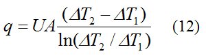
I went through my own heat exchanger design efforts when building a homemade air conditioner some time ago. It was a fun project which gave me a good practical understanding of how heat exchangers work. My first build attempt is shown in the two pictures below.
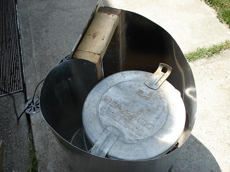
The picture above shows the inside of the unit. Air blows through the annular space and around a cold ice-water filled metal pail, causing the air to cool down before exiting through a hole at the top. Temperature measurements revealed that the air came out about 2.5 degrees Celsius cooler than it was going in. The heat exchange taking place is between the ice-water and the air. Naturally I want the heat exchange to be as high as possible so that the air comes out as cool as possible. So the task of figuring out how to do this is a heat exchanger problem.
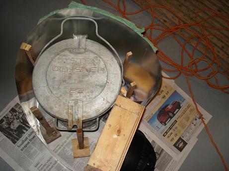
For my second attempt I added vertical wooden rods in the flow stream which helped to induce turbulent mixing which boosted heat transfer between the ice-water and air stream. This is shown in the picture below. The result was that the air came out about 3 degrees Celsius cooler, which is a slight improvement.
Not being satisfied with the result I decided to change the design completely. In this design (shown below) I made a U-shaped channel, which worked much better. Temperature measurements revealed that the exiting air was about 10 degrees Celsius cooler than it was going in, which is a great improvement over the earlier design.
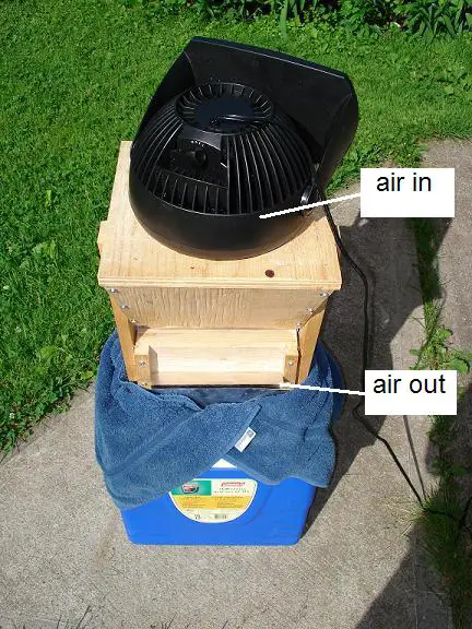
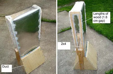
The picture above shows the U-shaped channel I made out of thin aluminum sheet, wood, and lots of silicone sealant around the edges so that water doesn't leak in when immersed in the ice-water. The channel has about a 1.8 cm gap through which the air flows. The width of the channel is 25 cm, and the length of the channel (i.e. the flow length along the U-shape) is about 60 cm. The U-shaped channel sits in a cooler of ice-water and the fan sits on top of the duct which has a hole in it so that the fan sits in snugly.
However, the household fan has difficulty blowing air through the narrow and long gap of the U-channel. The greatly improved heat transfer (and increased cooling of the air) resulting from the narrower and longer gap means that significant back pressure is created, which results in the fan having a much harder time pushing the air through the channel. The fan speed has to be set at the highest setting to get a decent rate of air flow through the channel. This is the tradeoff mentioned earlier between greater pressure drop and the increased heat transfer that results. Physically speaking, the fan must overcome the resistance to air flow associated with the pressure drop caused by the narrow and long gap the air must travel through. In this case it would be better to use a blower of some sort which is designed to push air in the presence of back pressure.
Return to Engineering page
Return to Real World Physics Problems home page
Free Newsletter
Subscribe to my free newsletter below. In it I explore physics ideas that seem like science fiction but could become reality in the distant future. I develop these ideas with the help of AI. I will send it out a few times a month.