About me and why I created this physics website.

Gyroscope Physics

Gyroscope physics is one of the most difficult concepts to understand in simple terms. When people see a spinning gyroscope precessing about an axis, the question is inevitably asked why that happens, since it goes against intuition. But as it turns out, there is a fairly straightforward way of understanding the physics of gyroscopes without using a lot of math.

But before I get into the details of that, it's a good idea to see how a gyroscope works (if you haven't already). Check out the video below of a toy gyroscope in action.




As you've probably noticed, a gyroscope can behave very similar to a spinning top. Therefore, the physics of gyroscopes can be applied directly to a spinning top.


To start off, let's illustrate a typical gyroscope using a schematic as shown below.



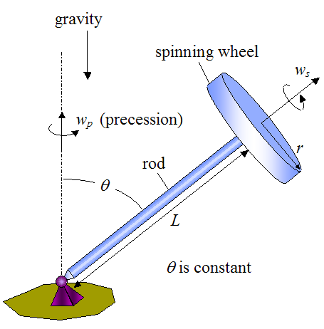
Where:

w_s is the constant rate of spin of the wheel, in radians/second

w_p is the constant rate of precession, in radians/second

L is the length of the rod

r is the radius of the wheel

θ is the angle between the vertical and the rod (a constant)


As the wheel spins at a rate w_s, the gyroscope precesses at a rate w_p about the pivot at the base (with θ constant).

The question is, why doesn't the gyroscope fall down due to gravity?!

The reason is this:

Due to the combined rotation w_s and w_p, the particles in the top half of the spinning wheel experience a component of acceleration a₁ normal to the wheel (with distribution as shown in the figure below), and the particles in the bottom half of the wheel experience a component of acceleration a₂ normal to the wheel in the opposite direction (with distribution as shown). Due to Newton’s second law, this means that a net force F₁ must act on the particles in the top half of the wheel, and a net force F₂ must act on the particles in the bottom half of the wheel. These forces act in opposite directions. Therefore a clockwise torque M is needed to sustain these forces. The force of gravity pulling down on the gyroscope creates the necessary clockwise torque M.



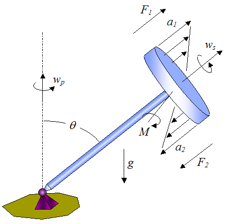
In other words, due to the nature of the kinematics, the particles in the wheel experience acceleration in such a way that the force of gravity is able to maintain the angle θ of the gyroscope as it precesses. This is the most basic explanation behind the gyroscope physics.

As an analogy, consider a particle moving around in a circle at a constant velocity. The acceleration of the particle is towards the center of the circle (centripetal acceleration), which is perpendicular to the velocity of the particle (tangent to the circle). This may seem counter-intuitive, but the lesson here is that the acceleration of an object can act in a direction that is very different from the direction of motion. This can result in some interesting physics, such as a gyroscope not falling over due to gravity as it precesses.


So now that we have an intuitive "feel" for the physics, we can analyze it in full using a mathematical approach. We will hence determine the equation of motion for the gyroscope.


Gyroscope Physics – Analysis

The general schematic for analyzing the physics is shown below.



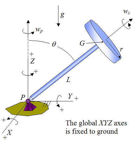
where g is the acceleration due to gravity, point G is the center of mass of the wheel, and point P is the pivot location at the base.

The global XYZ axes is fixed to ground and has origin at P.

I, J, and K are defined as unit vectors pointing along the positive X, Y, and Z axis respectively.

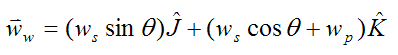
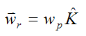
The angular velocity of the wheel, with respect to ground, is



The angular acceleration of the wheel, with respect to ground, is






Looking at the first term:




Looking at the second term:



Therefore,





The angular velocity of the rod, with respect to ground, is



The angular acceleration of the rod, with respect to ground, is zero since w_r is constant and does not change direction.


Note that the terms dJ/dt and dK/dt (given above) are calculated using vector differentiation. To learn more about it visit the vector derivative page.


     Wheel Analysis

Let's analyze the forces and moments acting on the wheel, due to contact with the rod. A free-body diagram of the wheel (isolated from the rod) is given below. Note that a local xyz axes is defined as shown, and is attached to the wheel so that it moves with the wheel, and has origin at point G.



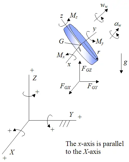
Where:

M_x is the moment acting in the local x-direction, at point G

M_y is the moment acting in the local y-direction, at point G

M_z is the moment acting in the local z-direction, at point G

F_GX is the force acting in the global X-direction, at point G

F_GY is the force acting in the global Y-direction, at point G

F_GZ is the force acting in the global Z-direction, at point G



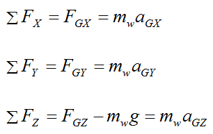
Apply Newton's Second Law to the wheel:



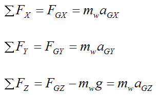
Where:

m_w is the mass of the wheel

a_GX is the acceleration of point G in the global X-direction

a_GY is the acceleration of point G in the global Y-direction

a_GZ is the acceleration of point G in the global Z-direction

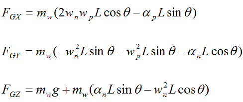
Since point G is traveling in a horizontal circle at constant velocity we have no tangential acceleration, so a_GX = 0, and F_GX = 0. So we only need to consider the second and third equation.

The second equation is,



Since point G is traveling in a horizontal circle at constant velocity we have centripetal acceleration. The centripetal acceleration points towards the center of rotation, therefore



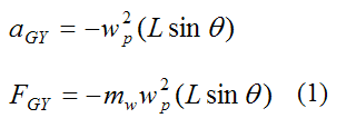
The third equation is,



Since point G is traveling in a horizontal circle at constant velocity we have a_GZ = 0. Thus,



Therefore,





Next, apply the Euler equations of motion for a rigid body, given that xyz is aligned with the principal directions of inertia of the wheel (treated as a solid disk).

We have,



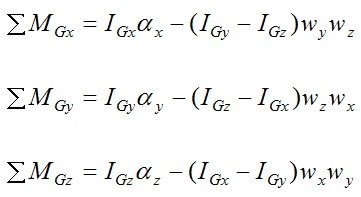
Now,



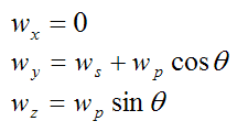
This is the angular velocity of the wheel (with respect to ground) resolved along the local xyz axes.

Furthermore,



This is the angular acceleration of the wheel (with respect to ground) resolved along the local xyz axes.

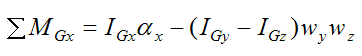
Thus, the second and third of Euler's equations are equal to zero, therefore ΣM_Gy = M_y = 0, and ΣM_Gz = M_z = 0. As a result, the second and third equations do not contribute to the solution. (Note that F_GX, F_GY, and F_GZ do not exert a moment (torque) about point G, since they are defined as coincident with point G - i.e. the length of the moment arm is zero).

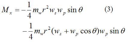
Therefore, we only need to consider the first equation:



Where:

ΣM_Gx is the sum of the moments about point G, in the local x-direction. Note that ΣM_Gx = M_x.

I_Gx, I_Gy, and I_Gz are the principal moments of inertia of the wheel about point G about the local x, y, and z directions (respectively).

By symmetry (treat the wheel as a thin circular disk),



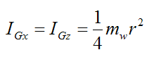
and



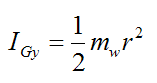
Therefore,




     Rod Analysis

Here we analyze the moments acting on the rod about point P. A free-body diagram of the rod (isolated from the wheel) is given below. Note that a local xyz axes is defined as shown, and is attached to the rod so that it moves with the rod, and has origin at point P. The xyz axes is aligned with the principal directions of inertia of the rod.



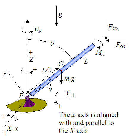
Note that point P is treated as a frictionless pivot. Therefore it exerts no moment (torque) on the rod. Since we are summing moments about P (which is a fixed point) we can use the moment (Euler) equations directly.



Now,



This is the angular velocity of the rod (with respect to ground) resolved along the local xyz axes, and



This is the angular acceleration of the rod (with respect to ground) resolved along the local xyz axes.

Thus, the second and third of Euler's equations are equal to zero, and they do not contribute to the solution.

Therefore, we only need to consider the first equation:



Where:

ΣM_Px is the sum of the moments about point P, in the local x-direction

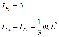
I_Px, I_Py, and I_Pz are the principal moments of inertia of the rod about point P about the local x, y, and z directions (respectively).

By symmetry,



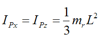
and



where m_r is the mass of the rod.

Therefore,




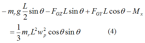
Combine equations (1)-(4) and we get:




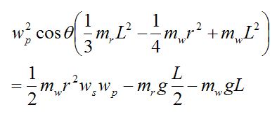
This is a nice compact equation. We can solve for any one of the values θ, w_p, or w_s if the other two values are known.

We can write a more general equation in which we replace the gyroscope wheel with any axisymmetric rotating body (with symmetry about the local y axis):



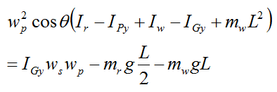
Where:



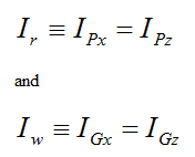
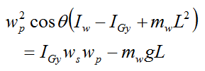
If we assume the mass of the rod is negligible, then m_r = I_r = I_Py = 0, and the above equation simplifies to a general equation for uniform gyroscopic motion with negligible rod mass:




In the next section we will look at gyroscopic stability, which is a very important and practical application of gyroscopes.


Gyroscopic Stability

From the angular momentum page we derived the following equation for a rigid body:



The term on the left is defined as the external impulse acting on the rigid body (between initial time t_i and final time t_f), due to the sum of the external moments (torque) acting on the rigid body. The terms on the right are the final angular momentum vector (H_f), and the initial angular momentum vector (H_i).

Although the above equation was derived for a rigid body it also applies to any system of particles (whether they comprise a rigid or non rigid body). The proof of this is commonly found in classical mechanics textbooks.

As is explained on the angular momentum page, the above equation applies for the two cases, where the local xyz axes has its origin at the center of mass G of the rigid body, or at a fixed point O on the rigid body (if there is one). In the remainder of this section, we will apply the former, so the moments, inertia terms, and angular momentum are all with respect to G.


To illustrate the concept of gyroscopic stability let's say we have an axisymmetric rigid object (such as a wheel) spinning in space with angular velocity w, at a given instant.



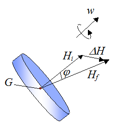
In the above figure, the change in the angular momentum vector between time t_i and t_f is given by ΔH, and according to the above equation ΔH is equal to the external impulse (due to the sum of the external moments acting between time t_i and t_f).

For a given ΔH (which is equal to the external impulse), the angle φ decreases as H_i increases. This means that the greater the magnitude of the initial angular momentum (H_i), the smaller the angle φ is for a given external impulse. Now, the magnitude of the angular momentum vector H is proportional to the magnitude of the angular velocity vector w. Therefore, the faster the object is spinning, the smaller the resulting angle φ is for a given external impulse.


If there are no external moments (torque) acting on the object then we say that the object is experiencing torque free motion. Thus, from the above equation, H_i = H_f, and φ = 0. Therefore, the angular momentum vector has constant magnitude and direction, and angular momentum is conserved.

For an axisymmetric rigid object experiencing torque free motion, the precession axis is seen (from the point of view of an observer) to coincide with the angular momentum vector, and this precession axis defines the average orientation of the object. And since this precession axis defines the average orientation of the object, then a small change in direction of the angular momentum vector (corresponding to a small φ, due to an external impulse) means a small change in the average orientation of the object. This of course means that after the external impulse is applied, the object is once again experiencing torque free motion.

Hence, a fast spinning axisymmetric object, experiencing torque free motion, is able to maintain its precession axis (and hence average orientation) with very little change, if an external impulse is applied.

Understanding the physics behind gyroscopes helps shed light on why mounting a spinning wheel (powered by a motor) onto a gimbal (metal frame) is so useful for navigation. The spinning wheel is mounted in the gimbal so as to be free of external torque. Therefore, given its already inherent orientation stability (as well as the fact that external torque is almost completely eliminated), the gyroscope experiences extremely little orientation change as a result. This is why gyroscopes are commonly used in navigation, such as in boats and ships. They tend to remain level even if the boat or ship changes orientation (either by pitching or rolling). The figure below illustrates a gyroscope-gimbal unit.




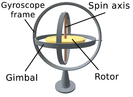
Source: http://en.wikipedia.org/wiki/Gyroscope. Author: http://en.wikipedia.org/wiki/User:Kieff/Gallery

Gyroscopic stability also explains why a spinning axisymmetric projectile, such as a football, can have its symmetric (long) axis stay aligned with its flight trajectory, without tumbling end over end when in flight. The spin imparts a gyroscopic response to the aerodynamic forces acting on the projectile, which results in the projectile long axis aligning itself with the flight trajectory. The physics involved here is a combination of gyroscopic analysis and aerodynamic force analysis due to drag and (potentially) the Magnus effect. This is quite complicated and will not be discussed here. However, there is a lot of literature available online on gyroscope physics, as related to projectile spin and gyroscopic stability, if one wishes to study this topic further.


Next in the analysis, we will show that for an axisymmetric rigid body experiencing torque free motion, the precession axis is seen (from the point of view of an observer in the inertial reference frame) to coincide with the angular momentum vector, which we know is fixed in inertial (ground) space, with constant magnitude and direction.


Torque Free Motion

Consider the figure below with local xyz axes as shown.



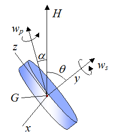
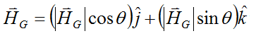
Let's find an equation that relates the angle θ (between H and w_s) to the vectors H and w_s. A simple way to do this is with the vector dot product:



Where:

H has been replaced with H_G (since we are using the angular momentum about the center of mass G of the object)

j is a unit vector pointing along the positive y axis

|H_G| is the magnitude of the vector H_G

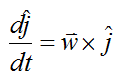
Differentiate the above equation with respect to time to give



which gives the following equation for dθ/dt:



From the vector derivative page we know that:





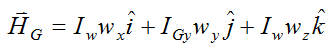
From the angular momentum page:



Where:

i, k are unit vectors pointing along the positive x and z axis, respectively

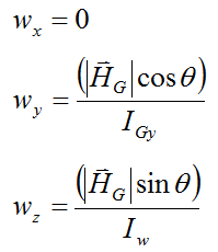
w_x, w_y, w_z are the components of the angular velocity vector of the object (with respect to ground), resolved along the x, y, z directions, respectively

I_x, I_y, I_z are the principal moments of inertia about the x, y, z directions, respectively

Substitute the above three equations into the equation for dθ/dt and we get



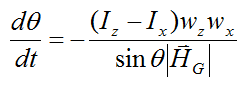
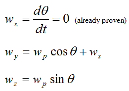
This is an informative equation coming out of the analysis done here. It tells us that for I_x = I_z, dθ/dt = 0 (as the object rotates through space). But if we choose α = 0 then the precession axis coincides with the angular momentum vector H_G, and as a result w_x = dθ/dt = 0 (which simplifies the calculations). Hence, the angle θ is constant and this is why, from the point of view of an observer in the inertial reference frame, the precession axis appears to coincide with the angular momentum vector. But mathematically speaking it does not matter what axis we choose as the precession axis, since it is simply a component of rotation. Being able to arbitrarily choose the precession axis is similar to how you can arbitrarily choose the x,y directions for a force calculation. Ultimately the answer is the same and the resultant force is not going to change. To understand this better you can read up on Euler angles which are commonly used to define the angular orientation of a body, using the concept of precession, spin, and nutation (which have been used in the analysis presented here).


Using the above result for I_x = I_z ≡ I_w, let's now find an equation relating w_s and w_p. Since θ is always constant we can express the angular momentum as follows in terms of its x,y,z components:



Now, from before



which can be written as (to match notation used previously):



We can equate the i,j,k components to give:



But from geometry we can also write:



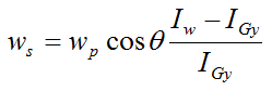
Solving the above equations for w_p and w_s we get



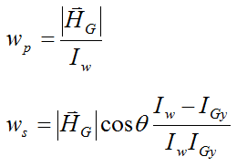
Hence, w_p and w_s are constant.

If we eliminate H_G from the above two equations we get



Note that this is the same as the equation given previously for uniform gyroscopic motion with negligible rod mass:



for the case L = 0. For L = 0, this equation reduces to torque free motion for an axisymmetric body.


The next section contains some additional information that is worth mentioning.


Gyroscope Physics – Additional Information


An axisymmetric object, experiencing torque free motion, that is experiencing pure spinning w_s about its symmetry axis (with no precession, w_p = 0) will have its angular momentum vector aligned with the spin axis, which is easy to understand. However, if this object is temporarily subjected to an external moment it will likely begin to precess as well as spin, and its (new) precession axis will coincide with the new angular momentum vector, which will no longer coincide with the spin axis. To calculate the new motion of the object due to the applied external moment, you need to solve the Euler equations of motion. These will allow you to mathematically determine the new quantities w_s, w_p, and θ, due to the applied external moment. After the external moment has been applied, these quantities will correspond to torque free motion.

In problems such as gyroscope physics analysis, solving the Euler equations of motion is necessary when moments are applied, since these equations directly account for them.


In torque free motion, the only external force acting on an object is at most gravity, which acts through the center of mass (G) of the object. The object is said to be experiencing torque free motion, since no torque (moment) is able to rotate the object about its center of mass, and thus the angular momentum about the center of mass does not change. It can therefore be assumed (for visualization purposes) that the center of rotation of the object is located at its center of mass G, since the angular momentum calculations (about G) are not affected by this assumption. This is why in torque free motion problems the angular velocity vector is typically shown passing through the center of mass of the object being analysed.


In the next section we will analyze a general case of gyroscope motion. This is undoubtedly very useful since it can apply to many different problems.


General Gyroscope Motion

In this final section we shall analyze a general case of gyroscope motion, as shown on the gyro top page. The gyro top shown there illustrates a state of general motion. The kinematic equations are already derived on the gyro top page so we can use those directly.

Assume that there is no friction anywhere.


     Wheel Analysis

From the gyro top page, the angular velocity of the gyroscope wheel is given by equation (1) on that page:



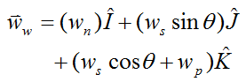
where the variables in this equation are defined in the gyro top page. Note that the term on the left has been replaced with w_w in order to match the notation used here.

From the gyro top page, the angular acceleration of the gyroscope wheel is given by equation (2) on that page:



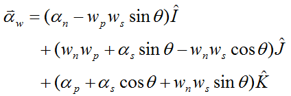
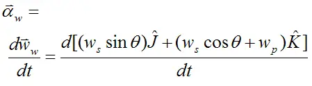
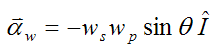
where the variables in this equation are defined in the gyro top page. Note that the term on the left has been replaced with α_w in order to match the notation used here.

From the gyro top page, point O on the wheel can be treated as the center of mass of the wheel (G). Therefore, for notation purposes, a_o on the left side of equation (5) on the gyro top page can be replaced with a_G.

After applying some considerable algebra to equation (5), and simplifying, we get the acceleration of the center of mass G of the gyroscope wheel:



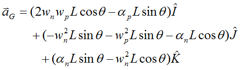
where the variables in this equation are defined in the gyro top page.

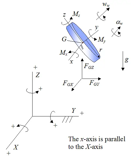
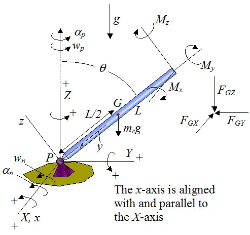
Consider next the following schematic of the gyroscope wheel (used previously), with variables previously defined. The same basic analysis as used before will be used here. Now, even though the gyroscope wheel rotates through space, the setup below can be used with local xyz always oriented as shown, for every stage of the motion. This can be done because the wheel is axisymmetric so that the principal moments of inertia do not change relative to xyz, as the wheel rotates.



By Newton's second law:



Substitute the acceleration terms for the center of mass G into the above three equations, and we get the following force equations for the gyroscope wheel:



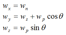
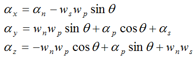
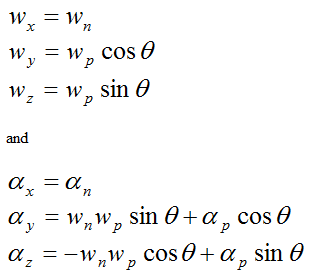
The angular velocity and angular acceleration of the gyroscope wheel is given with respect to the global XYZ axes. Using trigonometry we will resolve these onto the local xyz axes of the gyroscope wheel.

We get



and



Set



Apply the Euler equations of motion to the gyroscope wheel:




Next, consider the following schematic of the rod, with variables previously defined. The same basic analysis method as used before will be used here.


     Rod Analysis



Since the local xyz axes for the rod and wheel have the same orientation, we can find the resolved components of the angular velocity and angular acceleration of the rod by simply setting w_s = 0 and α_s = 0 in the equations for the angular velocity and angular acceleration of the wheel. This gives us



For the rod



Note that since point P is treated as a frictionless pivot it exerts no moment (torque) on the rod.

Since we are summing moments about P (which is a fixed point) we can use the moment (Euler) equations directly.



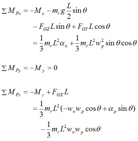
In the equation for ΣM_Py above, note that F_GX, F_GY, F_GZ, and gravity does not exert a moment about the local y axis.

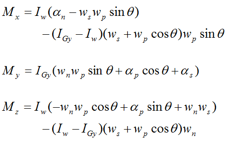
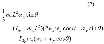
Substitute the force equations and Euler equations for the gyroscope wheel into the above three equations and simplify. We then get the final three equations with which to solve for the general gyroscope motion:





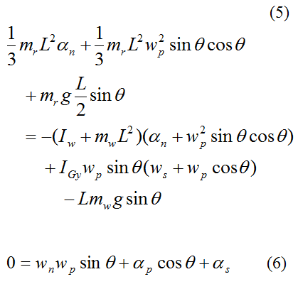
According to the sign convention used,



Let's assume we have a massless rod where m_r = 0.

We can rewrite equation (6) as



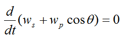
Therefore,



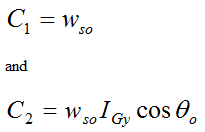
where C₁ is a constant.

We can rewrite equation (7) as



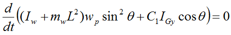
Therefore,



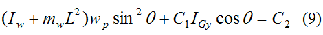
where C₂ is a constant.

From equations (8) and (9) we get



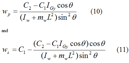
To solve this problem we first need to set boundary conditions. Let's choose the following.

For θ = θ_o, set w_n = w_p = 0, and w_s = w_so. This results in



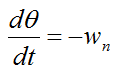
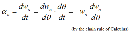
Substitute equation 10 (for w_p) into equation (5) and set



Simplify equation (5) and then perform (very tedious) integration to obtain an equation for w_n. We get



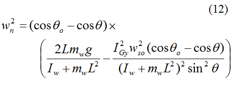
The angular velocities w_n, w_p, and w_s in equations 10-12 can be numerically integrated with respect to time to determine the corresponding orientation angles, as a function of time. The name given to these three orientation angles (corresponding to w_n, w_p, and w_s) is Euler angles, which are a common way to define the orientation of any rigid body in three-dimensional space.

Equations 10-12 mathematically describe the motion of any axisymmetric body attached to and rotating on a massless rod attached to a frictionless pivot, with axis of symmetry of the body pointing in the direction of the rod axis. These are undoubtedly a nice set of equations coming out of the analysis for general motion.

Equations 10-12 also apply for an axisymmetric top pivoted about point P, with point P lying on the symmetry axis. In this case L is the distance from point P to the center of mass G of the top. And the inertia terms are calculated about the center of mass G of the top (as was done for the gyroscope wheel).

The motion predicted by equations 10-12 is known as cuspidal motion, based on the boundary conditions given previously.


Closing Remarks

This completes the analysis. As you can see, gyroscope physics is a complex subject worthy of deeper understanding. It is hoped that you have gained a real sense of how gyroscopes work, as well as inspired some curiosity to look into them further on your own.

An intuitive explanation for gyroscopes was given near the start of the page. This explanation works well to explain how a gyroscope experiencing constant rates of precession and spin can maintain a constant angle θ. But in the analysis given above, the gyroscope first falls from angle θ_o and then starts to precess, while also experiencing cyclical angle change θ. Intuition fails to explain why this happens, which is often the case in physics when dealing with complex problems. But perhaps a decent explanation for this is to use a spring analogy. If a mass is hanging from a spring while in equilibrium, the vertical position of the mass will not change. But if that mass is raised and then released from rest it will oscillate vertically up and down. The system is no longer in equilibrium and the oscillatory motion is simply a physical way to "correct" an imbalance of forces. The same basic idea applies to a gyroscope that is released from rest, which can perhaps help you understand the physics taking place.



Return to Miscellaneous Physics page


Return to Real World Physics Problems home page