About me and why I created this physics website.
The Physics Of Volleyball
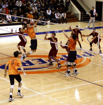
Source: http://www.flickr.com/photos/chrisamichaels/3230955360
Physics Of Volleyball – Optimizing The Serve
One way to optimize a volleyball serve is to minimize the time the ball spends in the air. This in turn minimizes the reaction time of the opposing team, making it more difficult for them to return the shot. In this analysis of the volleyball physics, we will look at ways to minimize the time the ball spends in the air, after the serve is made.
To set up this physics analysis we must first define the different variables in the problem. The schematic below shows a top view of a volleyball court, with labels given as shown.
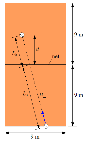
Where:
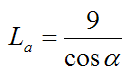
La is the distance from the serve location (behind the end line) to the net, along the direction the volleyball is served
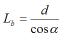
Lb is the arbitrary distance from the net to where the ball lands on the other side of the court, along the direction the volleyball is served
d is the distance beyond the net where the ball lands
α is the angle the volleyball trajectory makes with the side line
The following schematic shows a view of the volleyball trajectory, between the point of serve and the point at which the volleyball lands on the court.
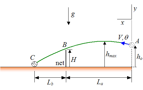
Where:
g is the acceleration due to gravity (equal to 9.8 m/s2 on earth)
H is the height of the net
hmax is the maximum height reached by the ball
ho is the initial height of the ball at the serve location
V is the initial serve velocity of the ball
θ is the initial angle the ball makes with the horizontal (and above it)
Point A is the serve location
Point B is the location just above the net, through which the ball passes
Point C is the location on the court where the ball lands
The coordinate system xy is defined with the positive x and y axes pointing in the directions shown. For convenience, the origin of this coordinate system is at point A.
The physics behind this analysis is of a kinematic nature, since we are only concerned with the motion of the ball. This optimization problem is an interesting application of projectile motion. To simplify this analysis we shall assume that air resistance and aerodynamic effects acting on the volleyball can be ignored.
From the equations for projectile motion, we have
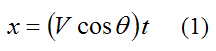
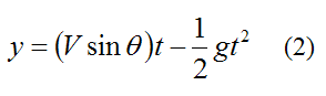
Where x and y denotes the position of the ball at any point in its trajectory, and t is time, in seconds.
Combine equations (1) and (2) to remove the time variable t and we get
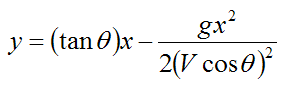
This is the equation of a parabola in terms of x and y. This equation has the general form:
Where:
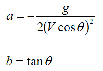
The variables a and b can be solved for in terms of the parameters La, Lb, ho, and H. They can be solved using two simultaneous equations based on the coordinates of points B and C, relative to the coordinate system xy (with origin at point A).
The coordinates of point B (relative to xy) is (La , H−ho)
The coordinates of point C (relative to xy) is (La+Lb , -ho)
Where:
The coordinates (x,y) for points B and C can be substituted for x and y in the general parabola equation given by
We can then solve for a and b in terms of the parameters La, Lb, ho, and H. These can then be used to solve for the initial velocity V and initial angle θ of the volleyball using the following equations:
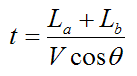
The time that the ball is airborne (i.e. the time we wish to minimize) is given by
Upon analysis of the results we find that we can minimize the time by doing three things:
(1) Get the ball just over the net
(2) Make Lb as large as possible (serve the ball so that it lands near the end line)
(3) Make ho as large as possible (with a jump serve)
Points (1) and (2) make sense since a shallower trajectory means the ball reaches a lower maximum height hmax, which means the ball spends less time in the air. However, if the ball lands close to the net (with small Lb), then the ball requires a high arc. This means that the ball is airborne for a longer period of time.
Point (3) makes sense since serving the ball at an ho as large as possible (with a jump serve), enables the ball to start its downward trajectory sooner (since hmax is reached sooner). This also decreases the time the ball spends in the air.
To get an idea of how much time the ball spends in the air, let's say we have d = 9 m, ho = 3.0 m, and H = 2.4 m. The time the ball spends in the air is t = 0.86 seconds.
A volleyball player can put the above three points into practice by practicing jump serves which (1) barely get the ball over the net, and (2) land as close as possible to the end line. The picture below shows an example of a jump serve.
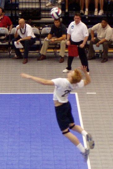
Source: http://en.wikipedia.org/wiki/Volleyball. Author: http://commons.wikimedia.org/wiki/User:Spangineer
In addition, serving the ball at a cross-court angle α does not change the time the ball spends in the air (for a given d, ho, and H). It only affects the horizontal speed of the ball (Vcosθ). So, the greater the angle α, the greater the ball speed. This can be advantageous since a higher serve velocity V can make it more difficult for the opposing team to return the shot.
The analysis shown previously allows us to predict the primary kinematic behaviour of a volleyball serve, subject to the assumption that air drag and aerodynamic effects can be ignored. However, these effects can in fact be significant and must be accounted for in order to make the model prediction as accurate as possible. In the next section we will discuss these effects in greater detail.
The Magnus Effect And Air Resistance
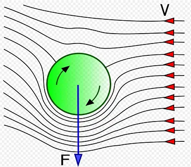
The airborne time of the volleyball can be reduced even more by putting top-spin on the volleyball. This causes the ball to experience an aerodynamic force known as the magnus effect, which "pushes" the ball downward so that it lands faster. This complicates the physics analysis. The figure below illustrates the magnus effect.
Source: http://en.wikipedia.org/wiki/Magnus_effect. Author: http://en.wikipedia.org/wiki/User:Gang65
As the ball spins, friction between the ball and air causes the air to react to the direction of spin of the ball.
As the ball undergoes top-spin (shown as clockwise rotation in the figure), it causes the velocity of the air around the top half of the ball to become less than the air velocity around the bottom half of the ball. This is because the tangential velocity of the ball in the top half acts in the opposite direction to the airflow, and the tangential velocity of the ball in the bottom half acts in the same direction as the airflow. In the figure shown, the airflow is in the leftward direction, relative to the ball.
Since the (resultant) air speed around the top half of the ball is less than the air speed around the bottom half of the ball, the pressure is greater on the top of the ball. This causes a net downward force (F) to act on the ball. This is due to Bernoulli's principle which states that when air velocity decreases, air pressure increases (and vice-versa).
As a result, by putting enough top-spin on the volleyball, the airborne time can be further reduced by as much as a tenth of a second. The following paper by D. Lithio and E. Webb explains the details of a volleyball serve and include mathematical models which account for the effects of air resistance (drag) and top-spin:
Optimizing A Volleyball Serve, Dan Lithio, Hope College, and Eric Webb, Case Western Reserve University, October 14, 2006.
This paper is very informative for those wishing to see the full analysis of the physics of volleyball, with regards to optimizing the serve.
Return to The Physics Of Sports page
Return to Real World Physics Problems home page